Quick Start Tutorial
This notebook shows an example Exploratory Data Analysis utilizing data-describe.
Note: Part of this notebook uses optional dependencies for text analysis. To install these dependencies, run pip install data-describe[nlp]
[1]:
import data_describe as dd
Data
This tutorial uses toy datasets from sklearn.
[2]:
from sklearn.datasets import load_boston
import pandas as pd
[3]:
dat = load_boston()
df = pd.DataFrame(dat['data'], columns=dat['feature_names'])
df['price'] = dat['target']
[4]:
df.head()
[4]:
| CRIM | ZN | INDUS | CHAS | NOX | RM | AGE | DIS | RAD | TAX | PTRATIO | B | LSTAT | price | |
|---|---|---|---|---|---|---|---|---|---|---|---|---|---|---|
| 0 | 0.00632 | 18.0 | 2.31 | 0.0 | 0.538 | 6.575 | 65.2 | 4.0900 | 1.0 | 296.0 | 15.3 | 396.90 | 4.98 | 24.0 |
| 1 | 0.02731 | 0.0 | 7.07 | 0.0 | 0.469 | 6.421 | 78.9 | 4.9671 | 2.0 | 242.0 | 17.8 | 396.90 | 9.14 | 21.6 |
| 2 | 0.02729 | 0.0 | 7.07 | 0.0 | 0.469 | 7.185 | 61.1 | 4.9671 | 2.0 | 242.0 | 17.8 | 392.83 | 4.03 | 34.7 |
| 3 | 0.03237 | 0.0 | 2.18 | 0.0 | 0.458 | 6.998 | 45.8 | 6.0622 | 3.0 | 222.0 | 18.7 | 394.63 | 2.94 | 33.4 |
| 4 | 0.06905 | 0.0 | 2.18 | 0.0 | 0.458 | 7.147 | 54.2 | 6.0622 | 3.0 | 222.0 | 18.7 | 396.90 | 5.33 | 36.2 |
Data Overview
CRIM per capita crime rate by town
ZN proportion of residential land zoned for lots over 25,000 sq.ft.
INDUS proportion of non-retail business acres per town
CHAS Charles River dummy variable (= 1 if tract bounds river; 0 otherwise)
NOX nitric oxides concentration (parts per 10 million)
RM average number of rooms per dwelling
AGE proportion of owner-occupied units built prior to 1940
DIS weighted distances to five Boston employment centres
RAD index of accessibility to radial highways
TAX full-value property-tax rate per $10,000
PTRATIO pupil-teacher ratio by town
B 1000(Bk - 0.63)^2 where Bk is the proportion of blacks by town
LSTAT % lower status of the population
MEDV Median value of owner-occupied homes in $1000’s
[5]:
df.shape
[5]:
(506, 14)
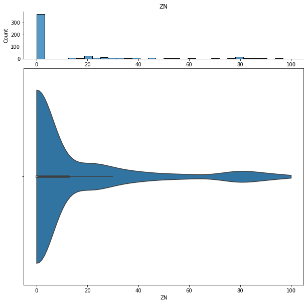
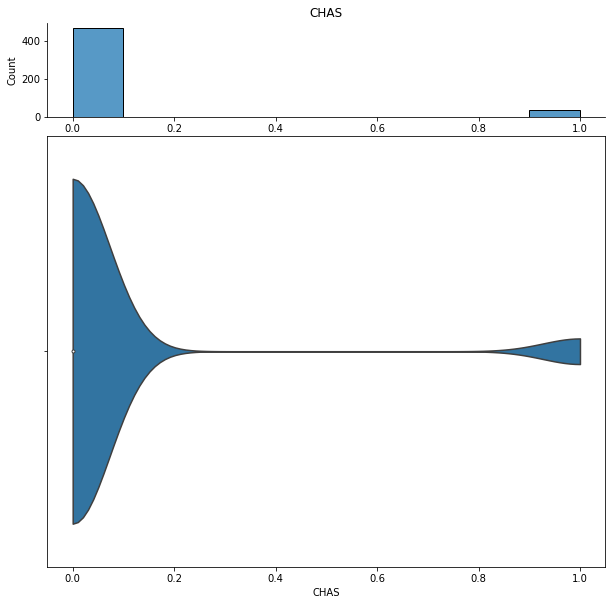
First we inspect some of the overall statistics about the data. Some examples of interesting things to note: - 93% of CHAS are the same value, zero - ZN also has a high amount of zeros - The mean of TAX is significantly higher than the median, suggesting this is right-skewed
[6]:
dd.data_summary(df)
| Info | |
|---|---|
| Rows | 506 |
| Columns | 14 |
| Size in Memory | 55.5 KB |
| Data Type | Nulls | Zeros | Min | Median | Max | Mean | Standard Deviation | Unique | Top Frequency | |
|---|---|---|---|---|---|---|---|---|---|---|
| CRIM | float64 | 0 | 0 | 0.0063 | 0.26 | 88.98 | 3.61 | 8.59 | 504 | 2 |
| ZN | float64 | 0 | 0 | 0 | 0 | 100 | 11.36 | 23.30 | 26 | 372 |
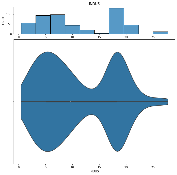
| INDUS | float64 | 0 | 0 | 0.46 | 9.69 | 27.74 | 11.14 | 6.85 | 76 | 132 |
| CHAS | float64 | 0 | 0 | 0 | 0 | 1 | 0.069 | 0.25 | 2 | 471 |
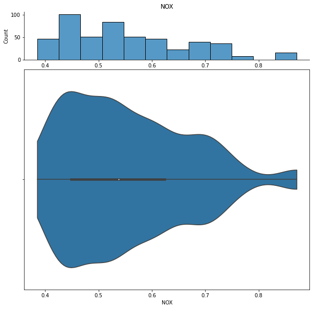
| NOX | float64 | 0 | 0 | 0.39 | 0.54 | 0.87 | 0.55 | 0.12 | 81 | 23 |
| RM | float64 | 0 | 0 | 3.56 | 6.21 | 8.78 | 6.28 | 0.70 | 446 | 3 |
| AGE | float64 | 0 | 0 | 2.90 | 77.50 | 100 | 68.57 | 28.12 | 356 | 43 |
| DIS | float64 | 0 | 0 | 1.13 | 3.21 | 12.13 | 3.80 | 2.10 | 412 | 5 |
| RAD | float64 | 0 | 0 | 1 | 5 | 24 | 9.55 | 8.70 | 9 | 132 |
| TAX | float64 | 0 | 0 | 187 | 330 | 711 | 408.24 | 168.37 | 66 | 132 |
| PTRATIO | float64 | 0 | 0 | 12.60 | 19.050 | 22 | 18.46 | 2.16 | 46 | 140 |
| B | float64 | 0 | 0 | 0.32 | 391.44 | 396.90 | 356.67 | 91.20 | 357 | 121 |
| LSTAT | float64 | 0 | 0 | 1.73 | 11.36 | 37.97 | 12.65 | 7.13 | 455 | 3 |
| price | float64 | 0 | 0 | 5 | 21.20 | 50 | 22.53 | 9.19 | 229 | 16 |
None
[6]:
data-describe Summary Widget
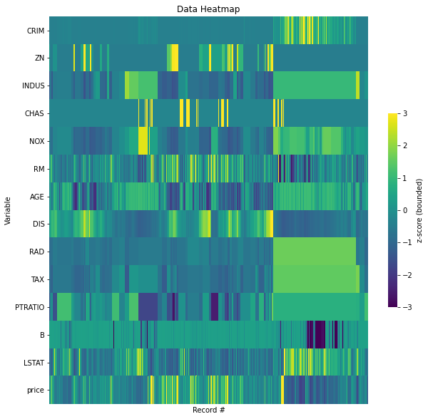
We can also look at a visual representation of the data as a heatmap:
[7]:
dd.data_heatmap(df)
[7]:
Heatmap Widget showing standardized values.
There are some sections of the data which have exactly the same values for some columns. For example, RAD = 1.661245 between record number 356 ~ 487. Similar patterns appear for INDUS and TAX. Is this a sorting issue or is there something else going on? Some additional investigation into data collection may answer these questions.
We can also look at the correlations:
[8]:
dd.correlation_matrix(df)
<AxesSubplot:title={'center':'Correlation Matrix'}>
[8]:
<data_describe.core.correlation.CorrelationWidget at 0x26b44cc2b48>
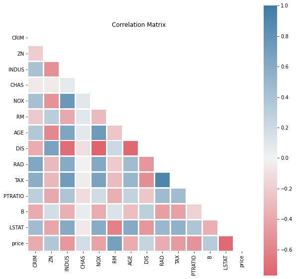
Features like AGE and DIS appear to be inversely correlated. CHAS doesn’t appear to have strong correlation with any other feature.
It might also help to re-order the features for comparisons using the cluster argument.
[9]:
dd.correlation_matrix(df, cluster=True)
<AxesSubplot:title={'center':'Correlation Matrix'}>
[9]:
<data_describe.core.correlation.CorrelationWidget at 0x26b44814f48>
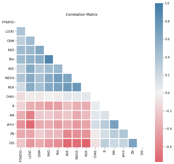
From this plot we can observe there are are two groups of inversely related features: PTRATIO to NOX and B to DIS.
Data Inspection
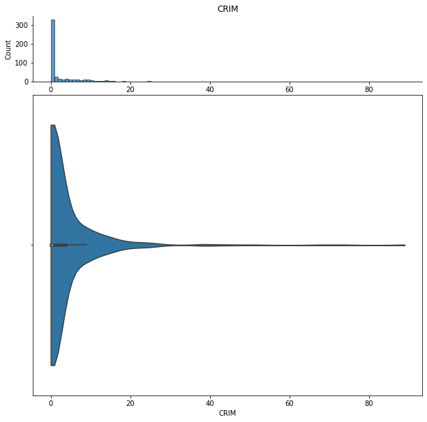
We can also do some more detailed inspection of individual features.
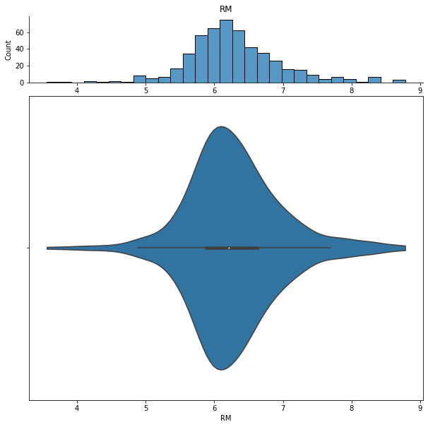
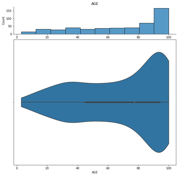
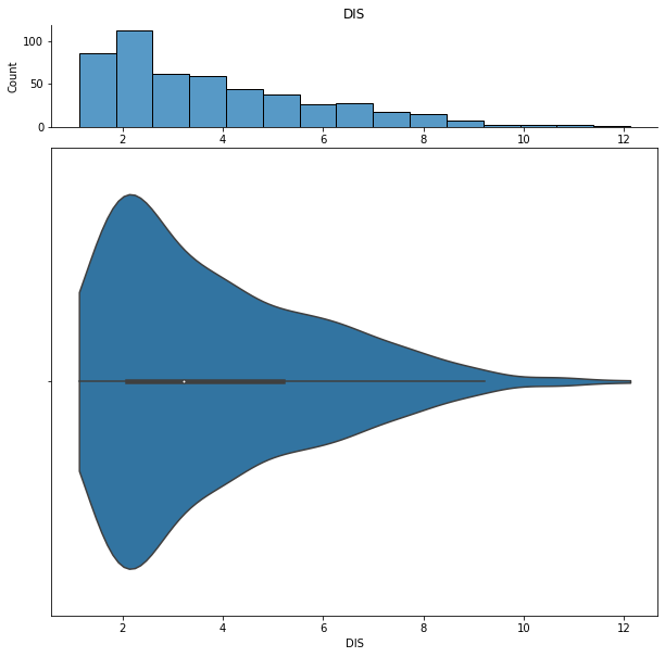
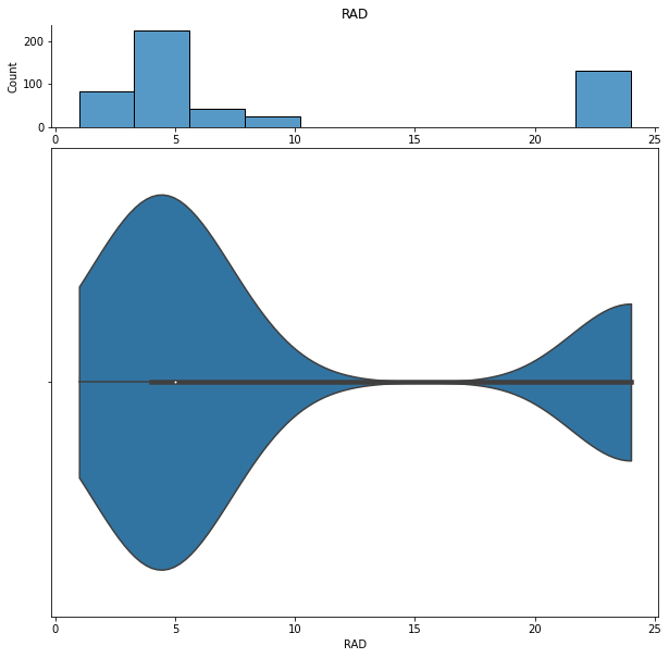
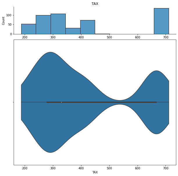
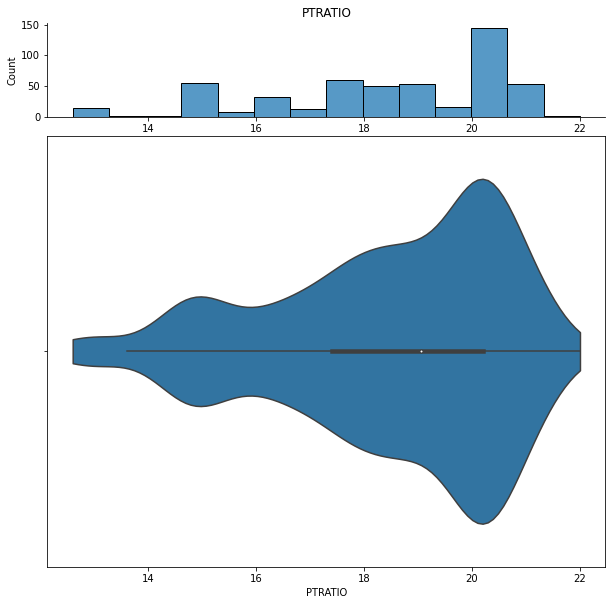
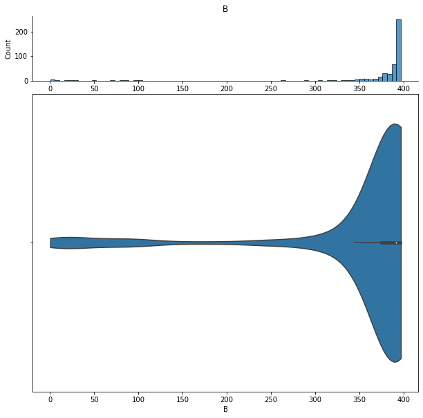
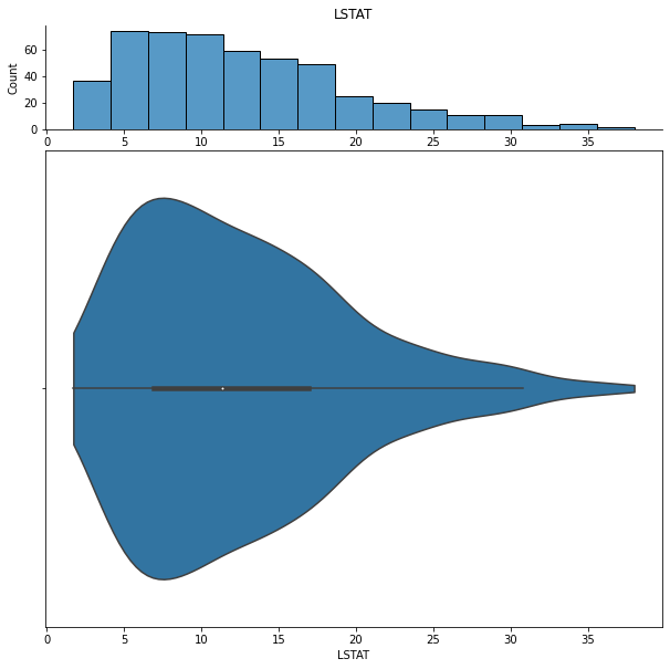
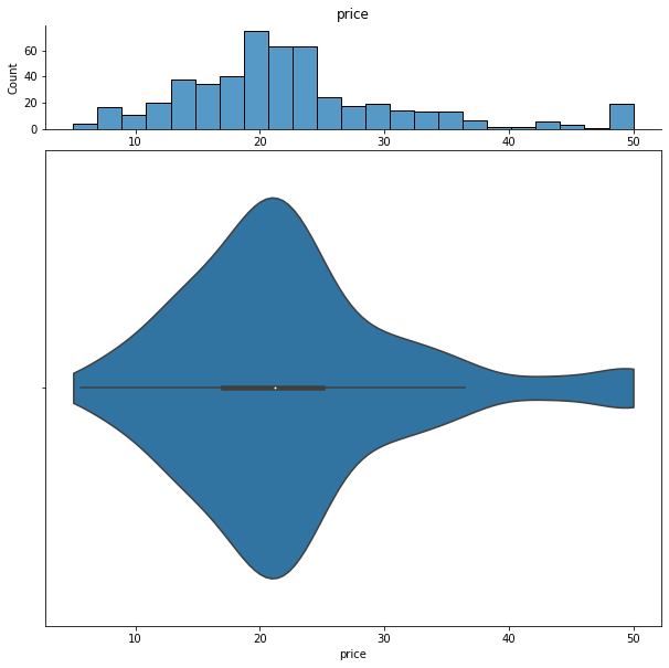
We can show histograms and violin plots of each numeric feature using the dd.distribution function.
[10]:
from IPython.display import display
# display is used to show plots from inside a loop
for col in df.columns:
    display(dd.distribution(df, plot_all=True).plot_distribution(col))
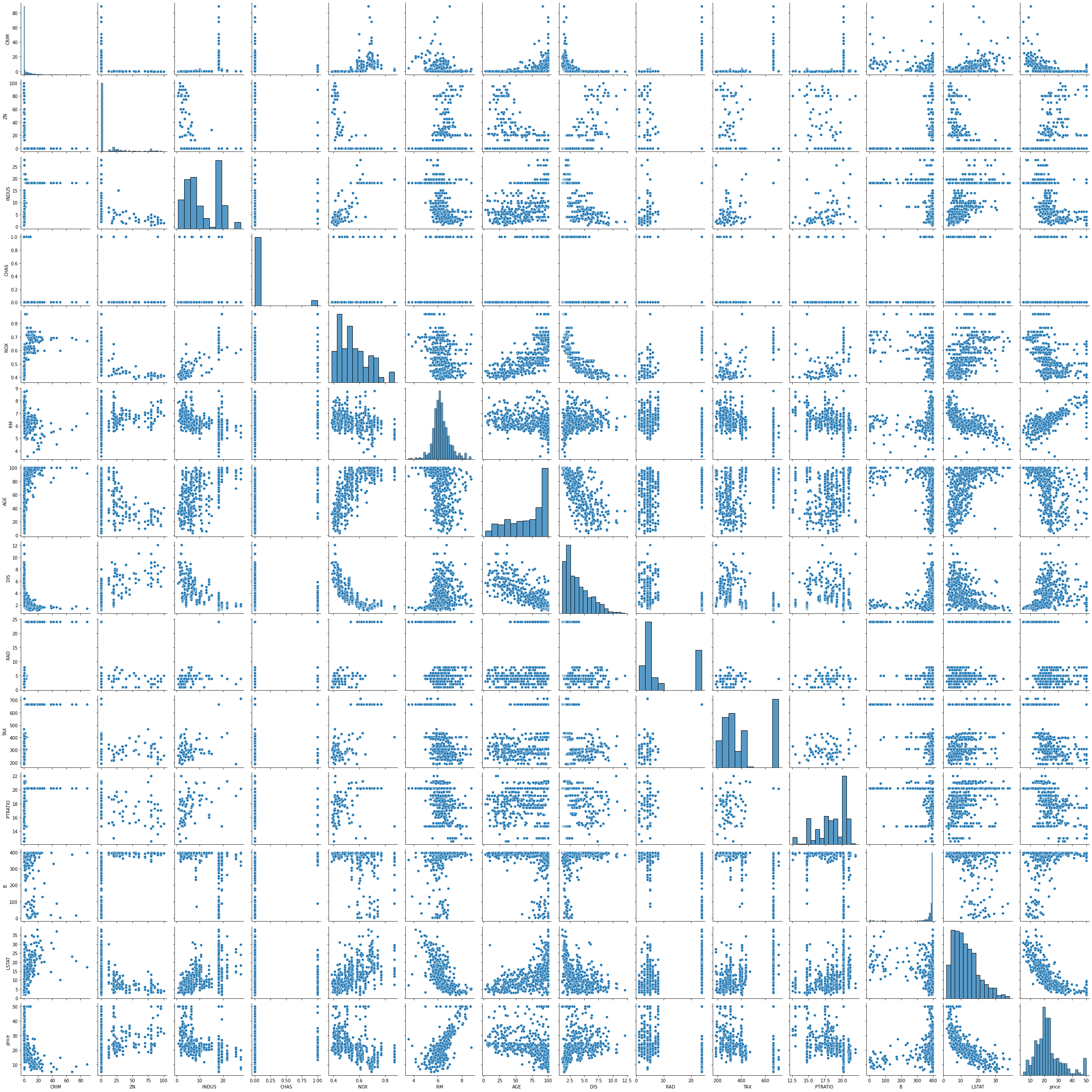
We can also look at bivariate distributions using scatter plots. In addition to plotting all pairs in a scatterplot matrix, we can also specify a filter for certain scatterplot diagnostic features.
[11]:
dd.scatter_plots(df, plot_mode='matrix')
<seaborn.axisgrid.PairGrid at 0x26b44e40188>
[11]:
data-describe Scatter Plot Widget

[12]:
dd.scatter_plots(df, threshold={'Outlier': 0.9})
<seaborn.axisgrid.PairGrid at 0x26b4dae2388>
[12]:
data-describe Scatter Plot Widget
Advanced Analysis
In addition to general plots, we can also use some advanced analyses as shown below.
Cluster Analysis
What segments or groups are present in the data?
[13]:
dd.cluster(df)
<AxesSubplot:title={'center':'kmeans Cluster'}, xlabel='Component 1 (47.0% variance explained)', ylabel='Component 2 (12.0% variance explained)'>
[13]:
Cluster Widget using kmeans
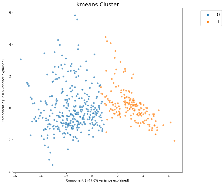
From this plot, we see that there does not appear to be strongly distinct clusters in the data.
Feature Importance
Which features are most predictive of price? We use Random Forest as a baseline model to test for importance.
[14]:
from sklearn.ensemble import RandomForestRegressor
[15]:
dd.importance(df, 'price', estimator=RandomForestRegressor(random_state=42))
[15]:
Text(0.5, 1.0, 'Feature Importance')
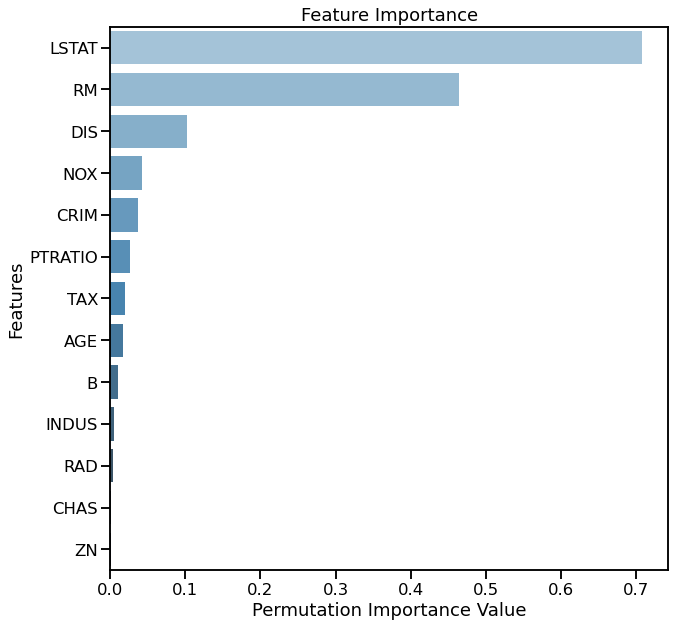
It appears that LSTAT and RM are most important for predicting price.
Topic Modeling
Since the Boston housing data set does not contain textual features, the 20 newsgroups text dataset is used to demonstrate the Topic Modeling widget.
[16]:
from sklearn.datasets import fetch_20newsgroups
[17]:
dat = fetch_20newsgroups(subset='test')
df2 = pd.DataFrame({'text': dat['data']})
df2 = df2.sample(150)
[18]:
df2.head()
[18]:
| text | |
|---|---|
| 1779 | From: penev@rockefeller.edu (Penio Penev)\nSub... |
| 5598 | From: mathew <mathew@mantis.co.uk>\nSubject: R... |
| 4313 | From: dps@nasa.kodak.com (Dan Schaertel,,,)\nS... |
| 97 | From: sinn@carson.u.washington.edu (Philip Sin... |
| 6225 | From: smn@netcom.com (Subodh Nijsure)\nSubject... |
Text preprocessing can be applied before topic modeling to improve accuracy.
[19]:
from data_describe.text.text_preprocessing import preprocess_texts, bag_of_words_to_docs
processed = preprocess_texts(df2['text'])
text = bag_of_words_to_docs(processed)
[20]:
from data_describe.text.topic_modeling import topic_model
[21]:
lda_model = topic_model(text, num_topics=3)
lda_model
| Topic 1 | Topic 1 Coefficient Value | Topic 2 | Topic 2 Coefficient Value | Topic 3 | Topic 3 Coefficient Value | |
|---|---|---|---|---|---|---|
| Term 1 | two | 0.023 | god | 0.045 | etc | 0.022 |
| Term 2 | use | 0.020 | us | 0.021 | help | 0.022 |
| Term 3 | .. | 0.018 | also | 0.017 | also | 0.022 |
| Term 4 | computer | 0.018 | use | 0.014 | two | 0.020 |
| Term 5 | anyone | 0.017 | work | 0.014 | may | 0.018 |
| Term 6 | right | 0.014 | way | 0.014 | back | 0.016 |
| Term 7 | think | 0.014 | see | 0.013 | think | 0.016 |
| Term 8 | game | 0.014 | many | 0.013 | make | 0.016 |
| Term 9 | system | 0.014 | think | 0.013 | take | 0.015 |
| Term 10 | way | 0.014 | well | 0.012 | well | 0.015 |
[21]:
<data_describe.text.topic_modeling.TopicModelWidget at 0x26b40933208>