Distributions

import pandas as pd
import data_describe as dd

from sklearn.datasets import load_boston
data = load_boston()
df = pd.DataFrame(data.data, columns=list(data.feature_names))
df['target'] = data.target

# Create categorical (bin) features to demonstrate count plots
df['AGE'] = df['AGE'].map(lambda x: "young" if x < 29 else "old")
df['CRIM'] = df['CRIM'].map(lambda x: "low" if x < df.CRIM.median() else "high")

df.head(2)

	CRIM	ZN	INDUS	CHAS	NOX	RM	AGE	DIS	RAD	TAX	PTRATIO	B	LSTAT	target
0	low	18.0	2.31	0.0	0.538	6.575	old	4.0900	1.0	296.0	15.3	396.9	4.98	24.0
1	low	0.0	7.07	0.0	0.469	6.421	old	4.9671	2.0	242.0	17.8	396.9	9.14	21.6

Diagnostic Summary

The default output summarizes diagnostics on the univariate data.

dist = dd.distribution(df)
dist

Distribution Summary:
        Skew detected in 1 columns.
        Spikey histograms detected in 0 columns.

        Use the method plot_distribution("column_name") to view plots for each feature.

        Example:
            dist = DistributionWidget(data)
            dist.plot_distribution("column1")

None

<data_describe.core.distributions.DistributionWidget at 0x1fa324be4c8>

Plot one feature

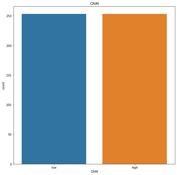
dist.plot_distribution("CRIM")

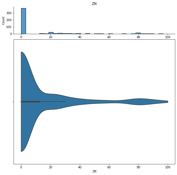
dist.plot_distribution("ZN")

import seaborn as sns
sns.__version__
# sns.displot(df, x="ZN", hue="CRIM")

'0.11.0'

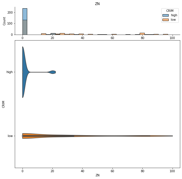
dist.plot_distribution("ZN", contrast="CRIM")

Display diagnostic values

dist.skew_value

ZN         2.219063
INDUS      0.294146
CHAS       3.395799
NOX        0.727144
RM         0.402415
DIS        1.008779
RAD        1.001833
TAX        0.667968
PTRATIO   -0.799945
B         -2.881798
LSTAT      0.903771
target     1.104811
dtype: float64